
Applying Conditional Formatting
Applying Conditional Formatting
You can apply conditional formatting, which can add color, text, or graphics to pivot table cells. To do so, you create rules that examine the values in the cells. This conditional formatting overrides any customization you added to the pivot table.
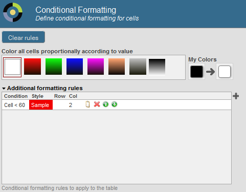
To do so, click the Conditional Formatting button  in the toolbar. The system displays a dialog box like the following (in this example, one rule has been specified):
Here, you can do the following:
-
Clear all conditional formatting. To do so, click Clear rules.
-
Apply an overall color, based on values in the cells. To do so, click a button in the section Color all cells proportionally according to value. See Applying an Overall Color.
-
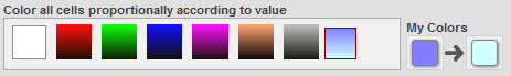
Define a custom gradient for use with the option Color all cells proportionally according to value. To define a custom gradient, use the two buttons displayed below My Colors. Click the first one and select a color to use at the bottom of the range. Click the second one and select a color to use at the top of the range. When you are done, the dialog box displays your gradient next to the predefined gradients. For example:
-
Create formatting rules. See Adding a Rule.
-
Change the order of the rules. To do so, click the up or down arrows in the row for a rule.
-
Delete a rule. To do so, click the X button in the row for that rule.
-
Reconfigure a rule. To do so, click the Reconfigure button
 in the row for that rule.
 -
Apply the existing rules while leaving this dialog box open. To do so, click Apply.
-
Apply the existing rules and exit this dialog box. To do so, click OK.
-
Close this dialog box without making changes. To do so, click Cancel.
Rules are applied in the same order that they are listed here. If a later rule contains formatting information that is inconsistent with an earlier rule, the system uses the formatting specified in the later rule.
Applying an Overall Color
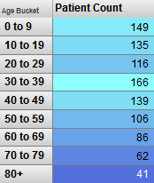
If you click a button in the section Color all cells proportionally according to value, the cells are colored according to their values. This works as follows: Each button displays a gradient of colors. To assign a color to a cell, the system examines the range of values of the cells. If a value is at the bottom of this range, the system uses the color that is shown at the top of the gradient button (a dark blue in the following example). If a value is at the top of this range, the system uses the color that is shown at the bottom of the gradient button (a light blue in the following example). For other values, the system uses an intermediate color. The following shows an example:
Adding a Rule
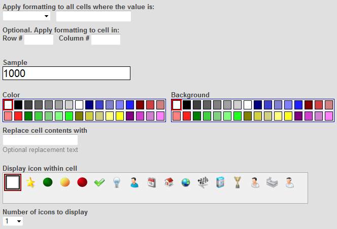
To add a rule, click the plus sign button. The system displays a dialog box where you can specify the rule details (in this example, one rule has been specified):
Here you can do the following:
-
Specify the numeric comparison for the rule to use. A rule compares the value in each cell (or in specific cells) to a constant, using an operator. For example:
cell_value > 50For each cell where this rule is true, the rule is applied. All the display details of the rule are applied to that cell.
To specify the numeric comparison, do the following:
-
Select an operator from the first drop-down menu.
-
Type a numeric constant into the field to the right of that.
-
-
Optionally specify which row, which column, or both the rule applies to. To do so, type a number into Row #, Col #, or both.
-
Optionally specify the text color to use when the rule is true. To do so, click a button in the Color section. If you select the left-most button, the system uses the default color.
-
Optionally specify the background color to use when the rule is true. To do so, click a button in the Background Color section. If you select the left-most button, the system uses the default color.
-
Optionally specify replacement text to display when the rule is true, instead of the actual cell value. To do so, type text into Replace cell contents with.
-
Optionally specify an icon to display when the rule is true, instead of the actual cell value. To do so, click a button in Display icon in cell. This area lists the system icons, followed by any custom icons defined by the implementers. (For information on adding icons that can be used here, see Creating Icons.)
If you select the left-most button, the system does not display an icon.
To display multiple icons, click a number from the Number of icons to display list.
The bottom of the dialog box shows a preview of the formatting.